Data visualisation: How weird is our jukebox?
28 Feb 2011
TechnologyOriginally posted at https://tech.labs.oliverwyman.com/blog/2011/02/28/data-visualisation-how-weird-is-our-jukebox/
One of the perennial unanswered questions among LShift hackers is “How weird is our jukebox?”. Not in the sense that it’s written in Erlang, but in the sense that we do play an awful lot of rather weird stuff on there.
The usual answer to this is “very”, but I’ve been thinking for a while about putting some numbers to it. The problem is that there’s no real standard for weirdness, nothing I can really use to establish which songs are odder than others (barring possibly some bleeding-edge music analysis, which isn’t really my field). I had an idea of something I could get at though that could serve as a stand-in: listener counts from last.fm.
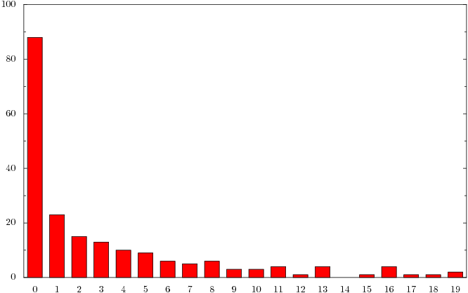
For a fairly “standard” user such as myself (a few bits of odd stuff, but a fair amount of more conventional fare in there as well), you get a graph that looks like this for my last 200 songs:
The numbers along the bottom don’t really mean anything, they’re just a set of equally sized “bins” for listener counts. The only problem is the bins are 30,000 listeners wide, and quite a lot of songs have less than that. In fact, this graph looks eerily like the classic Long Tail power law graph, and it’s shape doesn’t seem to vary very much between the various users I’ve tested this against.
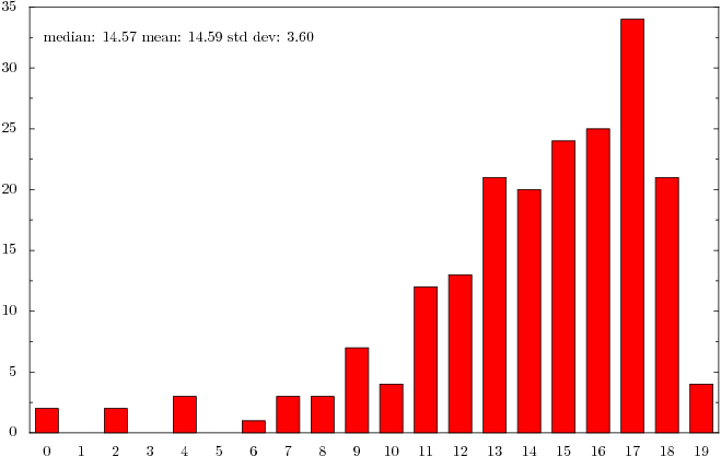
Dumping these numbers through a log function however gets us a slightly more useful graph.
The numbers along the bottom now have more of a meaning, in that they’re the rounded-down log2(x) values for each listener count. I’ve also thrown in the median/mean/standard deviation values for the graph. Between about 7 and 17 there’s a pretty clear popularity/listeners curve going on. I haven’t got much in the 19 group (which looks from staring at other values to be the highest any song on last.fm gets), and there’s a drop-off in 18, indicating I’m not listening to that much that’s really popular, but quite a lot that’s a little off that.
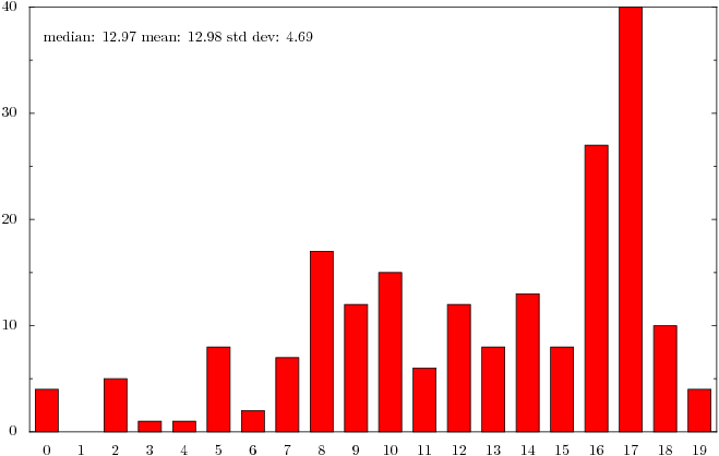
The LShift account paints a different picture
Again, we’ve got the peak at 17 (which I think is probably “alternative” music), but the drop-off after that is pretty dramatic, and there’s then a peak back again around 8-10. Remember, something in group 8 is on average 512 [(17-8)2] times less popular than group 17, so we’re drifting out of “selling lots of records” and down towards “we’re doing it for the art” territory. The spread here is significantly wider (see also standard deviation values of 4.69 v.s. my 3.6), indicating a wider selection of music with varying popularities.
So, in short, yes the LShift jukebox is notably weirder on average than my personal music tastes. Not quite sure how much weirder, but quite a lot! Although, now I’m being exposed to some new bits of music I hadn’t heard before, I’m starting to like a few new things and buying a few more things, so my weirdness values may increase a bit in the future…
As always, there’s a Github repo with all the code from here. “lastFMWeird.py” is the script you need for these examples, and it requires PyX to generate the graphs.


